38 excel pie chart add labels

How to Create and Format a Pie Chart in Excel - Lifewire Select the plot area of the pie chart. Right-click the chart. Select Add Data Labels . Select Add Data Labels. In this example, the sales for each cookie is added to the slices of the pie chart. Change Colors When a chart is created in Excel, or whenever an existing chart is selected, two additional tabs are added to the ribbon. Add / Move Data Labels in Charts - Excel & Google Sheets Add and Move Data Labels in Google Sheets. Double Click Chart. Select Customize under Chart Editor. Select Series. 4. Check Data Labels. 5. Select which Position to move the data labels in comparison to the bars.

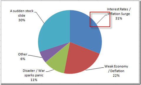
excel - How to not display labels in pie chart that are 0% - Stack Overflow Generate a new column with the following formula: =IF (B2=0,"",A2) Then right click on the labels and choose "Format Data Labels". Check "Value From Cells", choosing the column with the formula and percentage of the Label Options. Under Label Options -> Number -> Category, choose "Custom". Under Format Code, enter the following:

Excel pie chart add labels

45 Free Pie Chart Templates (Word, Excel & PDF) ᐅ TemplateLab Moreover, it’s also very easy to create a pie chart. You can do it by hand with the use of a mathematical compass and markers or pencils. For the tech-savvy, you can make a digital pie chart using a word processing software. Here are the steps to make a pie chart template using different methods: Using Microsoft Excel Add data labels and callouts to charts in Excel 365 - EasyTweaks.com Step #2: When you select the "Add Labels" option, all the different portions of the chart will automatically take on the corresponding values in the table that you used to generate the chart. The values in your chat labels are dynamic and will automatically change when the source value in the table changes. Step #3: Format the data labels. Pie of Pie Chart in Excel - Inserting, Customizing, Formatting Inserting a Pie of Pie Chart. Let us say we have the sales of different items of a bakery. Below is the data:-. To insert a Pie of Pie chart:-. Select the data range A1:B7. Enter in the Insert Tab. Select the Pie button, in the charts group. Select Pie of Pie chart in the 2D chart section.

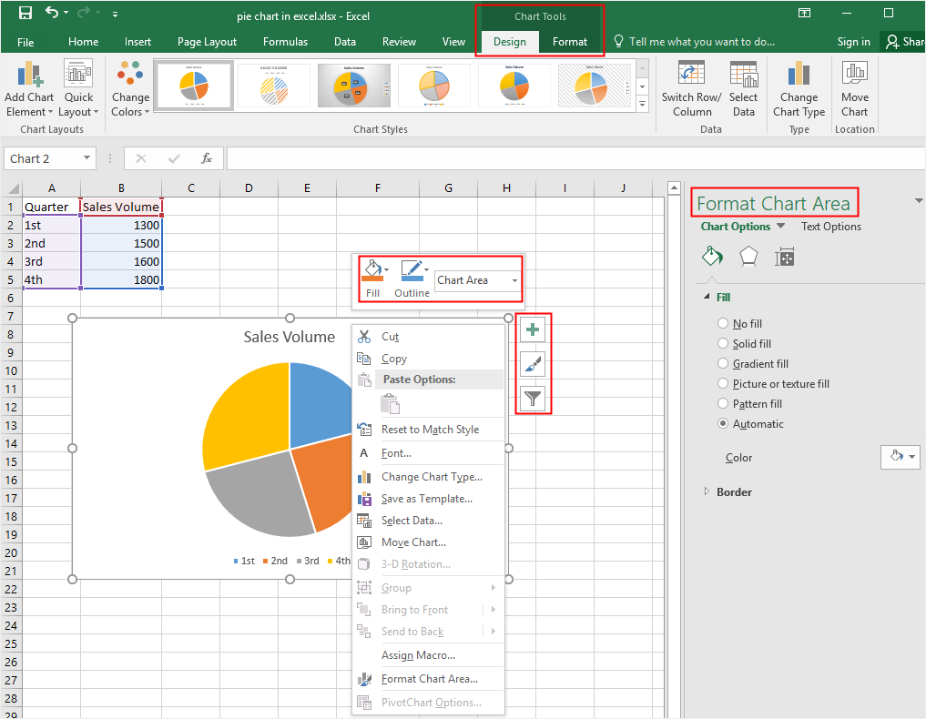
Excel pie chart add labels. Creating Pie Chart and Adding/Formatting Data Labels (Excel) Creating Pie Chart and Adding/Formatting Data Labels (Excel) Rotate charts in Excel - spin bar, column, pie and line ... Jul 09, 2014 · I think 190 degrees will work fine for my pie chart. After being rotated my pie chart in Excel looks neat and well-arranged. Thus, you can see that it's quite easy to rotate an Excel chart to any angle till it looks the way you need. It's helpful for fine-tuning the layout of the labels or making the most important slices stand out. Rotate 3-D ... c# - Add data labels to excel pie chart - Stack Overflow private void drawfractionchart (excel.worksheet activesheet, excel.chartobjects xlcharts, excel.range xrange, excel.range yrange) { excel.chartobject mychart = (excel.chartobject)xlcharts.add (200, 500, 200, 100); excel.chart chartpage = mychart.chart; excel.seriescollection seriescollection = chartpage.seriescollection (); excel.series … Adding 2nd Data Label Series to Bar of Pie Chart Re: Adding 2nd Data Label Series to Bar of Pie Chart. If you use 2 sets of the same data in the chart you can create 2 pie/bar charts, with one appearing on the secondary axis. Make sure the settings for bar/pie formatting are the same. Add data labels to each series. Format one to show names the other values.

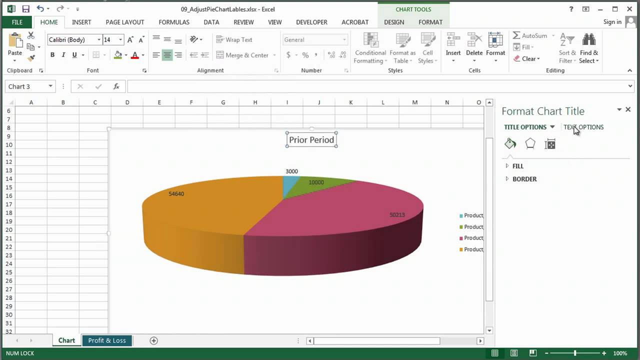
Edit titles or data labels in a chart - support.microsoft.com On a chart, click the label that you want to link to a corresponding worksheet cell. On the worksheet, click in the formula bar, and then type an equal sign (=). Select the worksheet cell that contains the data or text that you want to display in your chart. You can also type the reference to the worksheet cell in the formula bar. How-to Add Label Leader Lines to an Excel Pie Chart - YouTube Step-by-Step Tutorial: how-to create label leader lines that connect pie labels that are outsi... Map Chart in Excel | Steps to Create Map Chart in ... - EDUCBA Here you can customize the Fill color for this chart, or you can resize the area of this chart or add labels to the chart and the axis. See the supportive screenshot below: Step 9: Click on the navigation down arrow available besides the Chart Options. Add or remove data labels in a chart - support.microsoft.com Click the data series or chart. To label one data point, after clicking the series, click that data point. In the upper right corner, next to the chart, click Add Chart Element > Data Labels. To change the location, click the arrow, and choose an option. If you want to show your data label inside a text bubble shape, click Data Callout.

Pie Chart In Excel | Microsoft Excel Tips | Excel Tutorial | Free Excel ... Pie Chart In Excel Tutorial of pie chart's in Excel. A pie chart is often used at home, office and business. Its popularity comes mainly from the transparency of the presented data. A pie chart is best suited to show the data as part of a whole. | Microsoft Excel Tips | Excel Tutorial | Free Excel Help | Excel IF | Easy Excel No 1 Excel tutorial on the internet How to Add and Remove Chart Elements in Excel Select the data, go to insert menu --> Charts --> Line Chart. 1: Add Data Label Element to The Chart. To add the data labels to the chart, click on the plus sign and click on the data labels. This will ad the data labels on the top of each point. If you want to show data labels on the left, right, center, below, etc. click on the arrow sign. How to display leader lines in pie chart in Excel? - ExtendOffice To display leader lines in pie chart, you just need to check an option then drag the labels out. 1. Click at the chart, and right click to select Format Data Labels from context menu. 2. In the popping Format Data Labels dialog/pane, check Show Leader Lines in the Label Options section. See screenshot: 3. Adding data labels to a Pie Chart in VBA - Automate Excel VBA Code Examples for Excel. Excel. Formula Tutorials; Functions List. Excel Formulas Examples List. Excel Boot Camp. Shortcuts. Shortcut Training App; List of Shortcuts; Shortcut Coach. Charts. Chart Templates; Chart Add-in; Charts List; Excel VBA Consulting - Get Help & Hire an Expert!

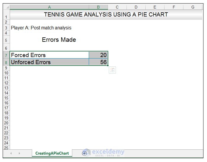
How to Make a Pie Chart in Excel & Add Rich Data Labels to The Chart!

Pie Chart in Excel - Inserting, Formatting, Filters, Data Labels To insert a Pie Chart, follow these steps:- Select the range of cells A1:B7 Go to Insert tab. In the charts group, Select the pie chart button Click on pie chart in 2D chart section. Adding Data Labels The default pie chart inserted in the above section is:-

How to Make a Pie Chart in Excel | EdrawMax Online

microsoft excel - How to make a Pie radar chart - Super User Dec 12, 2013 · Set the horizontal category axis labels to be your chart labels (G2:G9). Change the chart type for this new series to a pie chart. Remove the fill for the pie segments and add black borders. Add data labels for the pie series, selecting the Category Name instead of Value and setting the position to Outside End.

How to Add an Axis Title to an Excel Chart | Techwalla

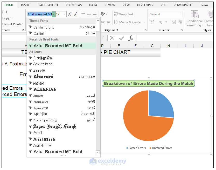
How to Make a Pie Chart in Excel & Add Rich Data Labels to The Chart! Creating and formatting the Pie Chart 1) Select the data. 2) Go to Insert> Charts> click on the drop-down arrow next to Pie Chart and under 2-D Pie, select the Pie Chart, shown below. 3) Chang the chart title to Breakdown of Errors Made During the Match, by clicking on it and typing the new title.

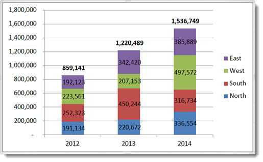
How to Show Percentages in Stacked Bar and Column Charts in Excel

How to Edit Pie Chart in Excel (All Possible Modifications) 9. Change Pie Chart's Legend Position. Just like the chart title and data labels, you can also edit a pie chart in Excel by changing the position of the legend. Follow the simple steps below to do this. 👇. Steps: Firstly, click on the chart area. Following, click on the Chart Elements icon.

How to Create and Label a Pie Chart in Excel 2013 : 8 Steps - Instructables

excel - How can I add labels with percentage to a pie chart in Python ... import matplotlib.pyplot as plt import pandas as pd excel_file_path = "Chartdata.xlsx" df = pd.read_excel(excel_file_path) df_country = df.groupby(['Country']).sum() df_country ['Revenue'].plot.pie() plt.show() It reads an Excel file, checks if there are more locations for one country and if yes, sums the revenues for the locations in the same ...

Creating Pie Chart and Adding/Formatting Data Labels (Excel) - YouTube

Inserting Data Label in the Color Legend of a pie chart Inserting Data Label in the Color Legend of a pie chart. Hi, I am trying to insert data labels (percentages) as part of the side colored legend, rather than on the pie chart itself, as displayed on the image below. Does Excel offer that option and if so, how can i go about it?

How-to Add Label Leader Lines to an Excel Pie Chart - Excel Dashboard Templates

Pie Chart in Excel | How to Create Pie Chart - EDUCBA Step 1: Select the data to go to Insert, click on PIE, and select 3-D pie chart. Step 2: Now, it instantly creates the 3-D pie chart for you. Step 3: Right-click on the pie and select Add Data Labels. This will add all the values we are showing on the slices of the pie.

30 Tableau Pie Chart Percentage Label - Label Design Ideas 2020

How to add axis label to chart in Excel? - ExtendOffice Add axis label to chart in Excel 2013 In Excel 2013, you should do as this: 1. Click to select the chart that you want to insert axis label. 2. Then click the Charts Elements button located the upper-right corner of the chart. In the expanded menu, check Axis Titles option, see screenshot: 3.

32 How To Label A Pie Chart In Excel - Labels Information List

Microsoft Excel Tutorials: Add Data Labels to a Pie Chart To add the numbers from our E column (the viewing figures), left click on the pie chart itself to select it: The chart is selected when you can see all those blue circles surrounding it. Now right click the chart. You should get the following menu: From the menu, select Add Data Labels. New data labels will then appear on your chart:

How to Adjust Pie Chart Labels in Excel : MS Excel Tips - YouTube

Stacked Column Chart in Excel (examples) - EDUCBA Pros of using Stacked Column Chart in Excel. They help in easily knowing the contribution of a factor to the group. They are easy to understand. Easy to visualize results on bar graphs. Easy to depict the difference between the various inputs of the same group. Cons of using Stacked Column Chart in Excel

How to Create and Format a Pie Chart in Excel

How to Create Pie Charts in Excel: The Ultimate Guide How to Add Labels to a Pie Chart in Excel. Adding labels to a pie chart is a great way to provide additional information about the data in the chart. To add click format data labels, select the pie chart and then go to the ribbon and click on the Add Data Labels button. This will add data labels for each pie chart slice that show the value of ...

How to Make a Pie Chart in Excel & Add Rich Data Labels to The Chart!

Doughnut Chart in Excel | How to Create ... - WallStreetMojo Doughnut Chart is a part of a Pie chart in excel Pie Chart In Excel Making a pie chart in excel can help you with the pictorial representation of your data and simplifies the analysis process. There are multiple kinds of pie chart options available on excel to serve the varying user needs. read more. A pie occupies the entire chart, but it will ...

How to display leader lines in pie chart in Excel?

Adding data labels to a pie chart - Excel General - OzGrid Re: Adding data labels to a pie chart To include the percentages: Code .ApplyDataLabels Type:=xlDataLabelsShowLabelAndPercent I don't know how you will get them bold. Why not try recording a macro when you do that manually? That's how I found the code to show the labels. Just found it: Code .SeriesCollection (1).DataLabels.Font.FontStyle = "Bold"

How to Create and Label a Pie Chart in Excel 2013 : 8 Steps - Instructables

How to Insert Axis Labels In An Excel Chart | Excelchat We will go to Chart Design and select Add Chart Element Figure 6 - Insert axis labels in Excel In the drop-down menu, we will click on Axis Titles, and subsequently, select Primary vertical Figure 7 - Edit vertical axis labels in Excel Now, we can enter the name we want for the primary vertical axis label.

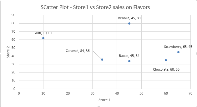
Add Custom Labels to x-y Scatter plot in Excel - DataScience Made Simple

Excel charts: add title, customize chart axis, legend and data labels ... Click the Chart Elements button, and select the Data Labels option. For example, this is how we can add labels to one of the data series in our Excel chart: For specific chart types, such as pie chart, you can also choose the labels location. For this, click the arrow next to Data Labels, and choose the option you want.

How to Make a Pie Chart in Excel & Add Rich Data Labels to The Chart!

Office: Display Data Labels in a Pie Chart - Tech-Recipes 3. In the Chart window, choose the Pie chart option from the list on the left. Next, choose the type of pie chart you want on the right side. 4. Once the chart is inserted into the document, you will notice that there are no data labels. To fix this problem, select the chart, click the plus button near the chart's bounding box on the right ...

How to Make a Pie Chart in Excel & Add Rich Data Labels to The Chart!

Pie of Pie Chart in Excel - Inserting, Customizing, Formatting Inserting a Pie of Pie Chart. Let us say we have the sales of different items of a bakery. Below is the data:-. To insert a Pie of Pie chart:-. Select the data range A1:B7. Enter in the Insert Tab. Select the Pie button, in the charts group. Select Pie of Pie chart in the 2D chart section.

Share :