42 how to add data labels to a pie chart in excel on mac

› 07 › 09Rotate charts in Excel - spin bar, column, pie and line charts Jul 09, 2014 · After being rotated my pie chart in Excel looks neat and well-arranged. Thus, you can see that it's quite easy to rotate an Excel chart to any angle till it looks the way you need. It's helpful for fine-tuning the layout of the labels or making the most important slices stand out. Rotate 3-D charts in Excel: spin pie, column, line and bar charts › 2014/01/20 › excel-chart-titleHow to add titles to Excel charts in a minute. - Ablebits.com Jan 20, 2014 · In Excel 2013 the CHART TOOLS include 2 tabs: DESIGN and FORMAT. Click on the DESIGN tab. Open the drop-down menu named Add Chart Element in the Chart Layouts group. If you work in Excel 2010, go to the Labels group on the Layout tab. Choose 'Chart Title' and the position where you want your title to display.

4 Ways To Add Data To An Excel Chart I said 4 ways so let's start with the first. 1. Copy Your Data & Click On Your Chart. So, let's add in some more data- another line in Row 10. Just copy the row data. Click on the outside of your chart. Hit Paste. Your chart will update. Easy as that.

How to add data labels to a pie chart in excel on mac

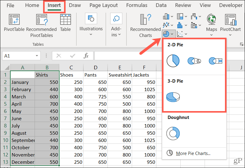
How to Use Cell Values for Excel Chart Labels - How-To Geek Select the chart, choose the "Chart Elements" option, click the "Data Labels" arrow, and then "More Options.". Uncheck the "Value" box and check the "Value From Cells" box. Select cells C2:C6 to use for the data label range and then click the "OK" button. The values from these cells are now used for the chart data labels. Pie Chart in Excel | How to Create Pie Chart - EDUCBA Go to the Insert tab and click on a PIE. Step 2: once you click on a 2-D Pie chart, it will insert the blank chart as shown in the below image. Step 3: Right-click on the chart and choose Select Data. Step 4: once you click on Select Data, it will open the below box. Step 5: Now click on the Add button. it will open the below box. Inserting pie chart in excel - EilidhMelodi Adding Data Labels The default pie chart inserted in the above section is- From this. Now from the Insert tab you need to select Insert Pie or Doughnut Chart. ... To create a pie chart in Excel 2016 add your data set to a worksheet and highlight it. Then click the Insert tab and click the dropdown menu next to the image of a pie chart. The ...

How to add data labels to a pie chart in excel on mac. How to Create a Pie Chart in Excel | Smartsheet To create a pie chart in Excel 2016, add your data set to a worksheet and highlight it. Then click the Insert tab, and click the dropdown menu next to the image of a pie chart. Select the chart type you want to use and the chosen chart will appear on the worksheet with the data you selected. Formatting data labels and printing pie charts on Excel for Mac 2019 ... Here's a work around I found for printing pie charts. Still can't find a solution for formatting the data labels. 1. When printing a pie chart from Excel for mac 2019, MS instructions are to select the chart only, on the worksheet > file > print. Excel is supposed to print the chart only (not the data ) and automatically fit it onto one page. › graphs › pie-chartsFree Pie Chart Maker - Make a Pie Chart in Canva Skip the complicated calculations – with Canva’s pie chart generator, you can turn raw data into a finished pie chart in minutes. A simple click will open the data section where you can add values. You can even copy and paste the data from a spreadsheet. Click the text to edit the labels. How to format the data labels in Excel:Mac 2011 when showing a ... Try clicking on Column or Row you want to set. Go to Format Menu; Click cells ; Click on Currency; Change number of places to 0 (zero) (if in accounting do the same thing. _____ Disclaimer: The questions, discussions, opinions, replies & answers I create, are solely mine and mine alone, and do not reflect upon my position as a Community Moderator.

How to Insert Axis Labels In An Excel Chart | Excelchat We will again click on the chart to turn on the Chart Design tab. We will go to Chart Design and select Add Chart Element. Figure 6 - Insert axis labels in Excel. In the drop-down menu, we will click on Axis Titles, and subsequently, select Primary vertical. Figure 7 - Edit vertical axis labels in Excel. Now, we can enter the name we want ... › Make-a-Pie-Chart-in-ExcelHow to Make a Pie Chart in Excel: 10 Steps (with Pictures) Apr 18, 2022 · Click the "Pie Chart" icon. This is a circular button in the "Charts" group of options, which is below and to the right of the Insert tab. You'll see several options appear in a drop-down menu: 2-D Pie - Create a simple pie chart that displays color-coded sections of your data. 3-D Pie - Uses a three-dimensional pie chart that displays color ... How to Add Axis Labels in Excel Charts - Step-by-Step (2022) - Spreadsheeto How to add axis titles 1. Left-click the Excel chart. 2. Click the plus button in the upper right corner of the chart. 3. Click Axis Titles to put a checkmark in the axis title checkbox. This will display axis titles. 4. Click the added axis title text box to write your axis label. How to Make a Pie Chart in Excel - Fireside Grill and Bar It's at the top of the Excel window, just right of the Home tab. Click the "Pie Chart" icon. This is a circular button in the "Charts" group of options, which is below and to the right of the Insert tab. You'll see several options appear in a drop-down menu: 2-D Pie - Create a simple pie chart that displays color-coded sections of your data.

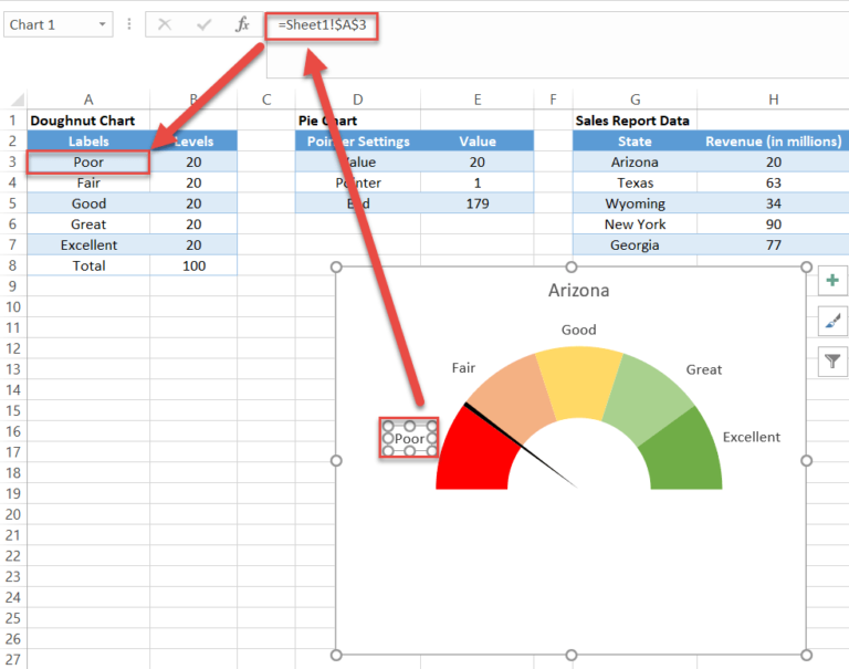
How to add or move data labels in Excel chart? - ExtendOffice In Excel 2013 or 2016. 1. Click the chart to show the Chart Elements button . 2. Then click the Chart Elements, and check Data Labels, then you can click the arrow to choose an option about the data labels in the sub menu. See screenshot: In Excel 2010 or 2007. 1. click on the chart to show the Layout tab in the Chart Tools group. See screenshot: 2. Then click Data Labels, and select one type of data labels as you need. See screenshot: Office: Display Data Labels in a Pie Chart - Tech-Recipes: A Cookbook ... 2. If you have not inserted a chart yet, go to the Insert tab on the ribbon, and click the Chart option. 3. In the Chart window, choose the Pie chart option from the list on the left. Next, choose the type of pie chart you want on the right side. 4. Once the chart is inserted into the document, you will notice that there are no data labels. support.microsoft.com › en-us › officeAdd or remove data labels in a chart - support.microsoft.com For example, in the pie chart below, without the data labels it would be difficult to tell that coffee was 38% of total sales. Depending on what you want to highlight on a chart, you can add labels to one series, all the series (the whole chart), or one data point. Add data labels. You can add data labels to show the data point values from the ... › charts › gauge-templateExcel Gauge Chart Template - Free Download - How to Create Step #7: Add the pointer data into the equation by creating the pie chart. Step #8: Realign the two charts. Step #9: Align the pie chart with the doughnut chart. Step #10: Hide all the slices of the pie chart except the pointer and remove the chart border. Step #11: Add the chart title and labels.

How to Make a Pie Chart in Microsoft Excel

How to add data labels from different column in an Excel chart? This method will guide you to manually add a data label from a cell of different column at a time in an Excel chart. 1. Right click the data series in the chart, and select Add Data Labels > Add Data Labels from the context menu to add data labels. 2. Click any data label to select all data labels, and then click the specified data label to select it only in the chart.

Excel Gauge Chart Template - Free Download - How to Create

How to Add New Extra Data to Existing Excel Chart (Easy) Add New Data to Existing Chart of Excel 2003-2016 Facebook Page : on twitter: :...

31 How To Label Vertical Axis In Excel

How to Add Data Labels to an Excel 2010 Chart - dummies Use the following steps to add data labels to series in a chart: Click anywhere on the chart that you want to modify. On the Chart Tools Layout tab, click the Data Labels button in the Labels group. A menu of data label placement options appears: None: The default choice; it means you don't want to display data labels.

31 How To Label Vertical Axis In Excel

How to Create Pie of Pie Chart in Excel? - GeeksforGeeks Follow the below steps to create a Pie of Pie chart: 1. In Excel, Click on the Insert tab. 2. Click on the drop-down menu of the pie chart from the list of the charts. 3. Now, select Pie of Pie from that list. Below is the Sales Data were taken as reference for creating Pie of Pie Chart:

35 Data Label Excel - Labels For Your Ideas

excel - How to set pie chart label format as a cellformat ... 2 You can link the number format of the labels to the number format of the cell. Via the UI you'd do this by formatting the labels and on the Number tab select "Link to source". If you run the macro recorder during that, you will get the respective VBA, i.e. link ActiveChart.SeriesCollection (1).DataLabels.NumberFormatLinked = -1 and unlink

29 Add Axis Label Excel Mac - 1000+ Labels Ideas

support.microsoft.com › en-us › officeChange the format of data labels in a chart You can add a built-in chart field, such as the series or category name, to the data label. But much more powerful is adding a cell reference with explanatory text or a calculated value. Click the data label, right click it, and then click Insert Data Label Field. If you have selected the entire data series, you won't see this command.

34 How To Label Graphs In Excel - Labels Design Ideas 2020

How to Make a PIE Chart in Excel (Easy Step-by-Step Guide) Once you have the data in place, below are the steps to create a Pie chart in Excel: Select the entire dataset Click the Insert tab. In the Charts group, click on the 'Insert Pie or Doughnut Chart' icon. Click on the Pie icon (within 2-D Pie icons). The above steps would instantly add a Pie chart on your worksheet (as shown below).

How To Make A Cashier Count Chart In Excel : How to make an organizational chart - YouTube : Pie ...

Add a DATA LABEL to ONE POINT on a chart in Excel Steps shown in the video above: Click on the chart line to add the data point to. All the data points will be highlighted. Click again on the single point that you want to add a data label to. Right-click and select ' Add data label ' This is the key step! Right-click again on the data point itself (not the label) and select ' Format data label '.