43 multiple data labels excel pie chart

Pie Chart in Excel | How to Create Pie Chart - EDUCBA Step 1: Do not select the data; rather, place a cursor outside the data and insert one PIE CHART. Go to the Insert tab and click on a PIE. Step 2: once you click on a 2-D Pie chart, it will insert the blank chart as shown in the below image. Step 3: Right-click on the chart and choose Select Data. Step 4: once you click on Select Data, it will ... Move data labels - support.microsoft.com Right-click the selection > Chart Elements > Data Labels arrow, and select the placement option you want. Different options are available for different chart types. For example, you can place data labels outside of the data points in a pie chart but not in a column chart.

How to☝️Create a Pie of Pie Chart in Excel - SpreadsheetDaddy Start off by following the chart creation method as described below. Select your data. Navigate to the Insert menu. In the Chart submenu, click on Insert Pie or Doughnut Chart. Pick the Pie of Pie Chart type. Voila! With those few steps, you have added a Pie of Pie Chart to your worksheet.

Multiple data labels excel pie chart

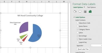
Excel Pie Chart Labels on Slices: Add, Show & Modify Factors - ExcelDemy The method to add category names to the data labels is given below step-by-step: 📌 Steps: First, double-click on the data labels on the pie chart. As a result, a side window called Format Data Labels will appear. Now, go to the drop-down of the Label Options to Label Options tab. Then, check the Category Name option. Everything You Need to Know About Pie Chart in Excel - SpreadsheetWeb How to Make a Pie Chart in Excel. Start with selecting your data in Excel. If you include data labels in your selection, Excel will automatically assign them to each column and generate the chart. Go to the INSERT tab in the Ribbon and click on the Pie Chart icon to see the pie chart types. Click on the desired chart to insert. How to Make a Pie Chart with Multiple Data in Excel (2 Ways) - ExcelDemy First, to add Data Labels, click on the Plus sign as marked in the following picture. After that, check the box of Data Labels. At this stage, you will be able to see that all of your data has labels now. Next, right-click on any of the labels and select Format Data Labels. After that, a new dialogue box named Format Data Labels will pop up.

Multiple data labels excel pie chart. Show multiple data lables on a chart - Power BI For example, I'd like to include both the total and the percent on pie chart. Or instead of having a separate legend include the series name along with the % in a pie chart. I know they can be viewed as tool tips, but this is not sufficient for my needs. Many of my charts are copied to presentations and this added data is necessary for the end ... How to group (two-level) axis labels in a chart in Excel? - ExtendOffice (1) In Excel 2007 and 2010, clicking the PivotTable > PivotChart in the Tables group on the Insert Tab; (2) In Excel 2013, clicking the Pivot Chart > Pivot Chart in the Charts group on the Insert tab. 2. In the opening dialog box, check the Existing worksheet option, and then select a cell in current worksheet, and click the OK button. 3. How to Show Percentage and Value in Excel Pie Chart - ExcelDemy Table of Contents hide. Download Practice Workbook. Step by Step Procedures to Show Percentage and Value in Excel Pie Chart. Step 1: Selecting Data Set. Step 2: Using Charts Group. Step 3: Creating Pie Chart. Step 4: Applying Format Data Labels. Conclusion. Related Articles. Formatting data labels and printing pie charts on Excel for Mac 2019 ... Here's a work around I found for printing pie charts. Still can't find a solution for formatting the data labels. 1. When printing a pie chart from Excel for mac 2019, MS instructions are to select the chart only, on the worksheet > file > print. Excel is supposed to print the chart only (not the data ) and automatically fit it onto one page.

How to create a chart in Excel from multiple sheets Nov 05, 2015 · If you want to plot data from multiple worksheets in your graph, repeat the process described in step 2 for each data series you want to add. When done, click the OK button on the Select Data Source dialog window. In this example, I've added the 3 rd data series, here's how my Excel chart looks now: 4. Customize and improve the chart (optional) Adding second set of data labels - Excel Help Forum Re: Adding second set of data labels. The chart links to workbooks on your hard drive, not to the data in the sheet. The secondary axis can only be shown when there is a series plotting on the secondary axis. Both your series are plotted on the first axis. You need to select the COUNT OF PARTS series, format it and send it to the secondary axis. Multiple Data Labels on a Pie Chart | MrExcel Message Board So I have a table with 8 rows and 3 columns. This table includes: Column 1 - shipment name Column 2 - shipment cost Column 3 - shipment weight I have created a pie chart from this table, which covers the first two columns. Displayed next to each slice is a label with the shipment name, shipment cost, and percent share of the pie. How to add data labels from different column in an Excel chart? This method will introduce a solution to add all data labels from a different column in an Excel chart at the same time. Please do as follows: 1. Right click the data series in the chart, and select Add Data Labels > Add Data Labels from the context menu to add data labels. 2.

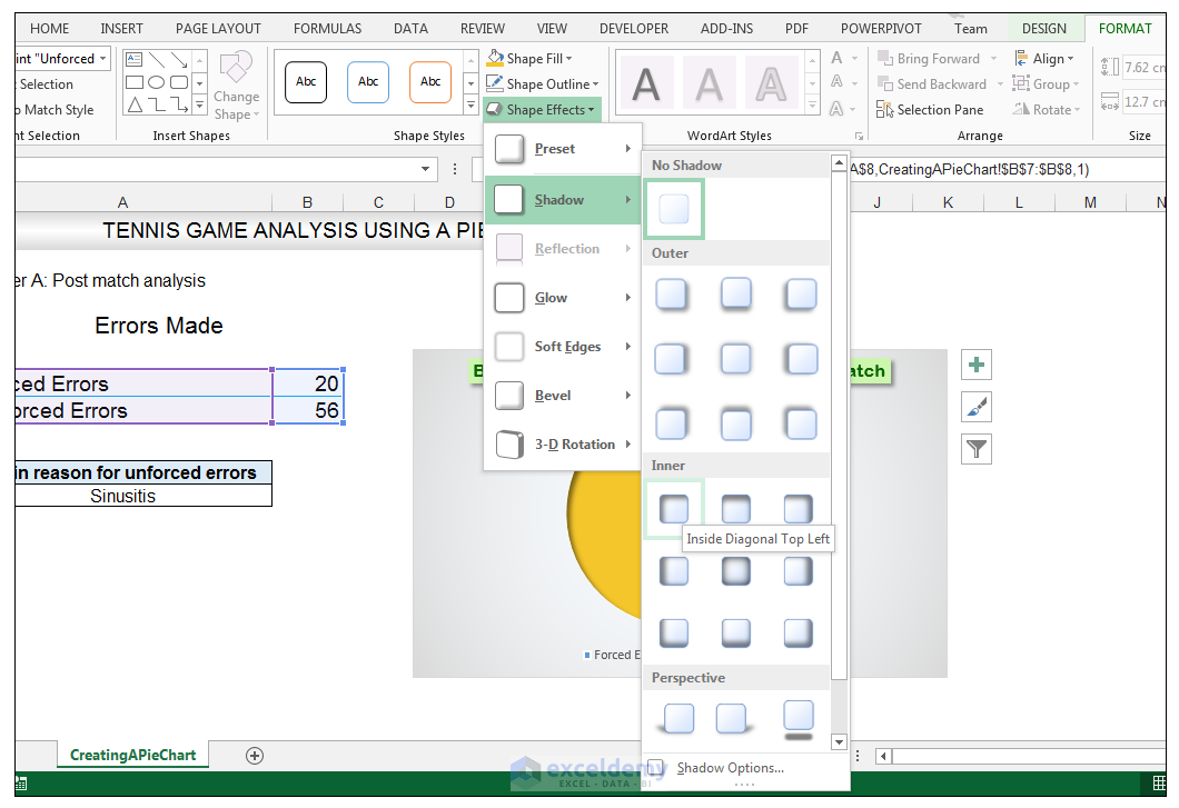
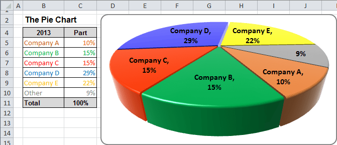
Pie Chart Examples | Types of Pie Charts in Excel with Examples To reduce the hole size, right-click on the chart, select the Format Data Series, and reduce the hole size. Try other options like color change, soften edges, doughnut explosion, etc., as per our requirement. Select all Data Labels at once - Microsoft Community AFAIK it has never been possible to select all data labels (if there are multiple series) You might be able to use code like this. Sub DL () Dim ocht As Chart Dim ser As Series Dim opt As Point Dim s As Long Dim p As Long Set ocht = ActiveWindow.Selection.ShapeRange (1).Chart For s = 1 To ocht.SeriesCollection.Count Multiple data labels (in separate locations on chart) Re: Multiple data labels (in separate locations on chart) You can do it in a single chart. Create the chart so it has 2 columns of data. At first only the 1 column of data will be displayed. Move that series to the secondary axis. You can now apply different data labels to each series. Attached Files 819208.xlsx‎ (13.8 KB, 265 views) Download How to Make a Pie Chart in Excel (Only Guide You Need) Jul 13, 2022 · Read More: How to Make Pie Chart in Excel with Subcategories (2 Quick Methods) Conclusion. Hope after reading this article you will not face any difficulties with the pie chart. This article covers all the necessary things regarding Excel Pie Chart. Stay tuned for more useful articles. Let us know what problems do you face with Excel Pie Chart.

Excel 3-D Pie Charts - Microsoft Excel undefined

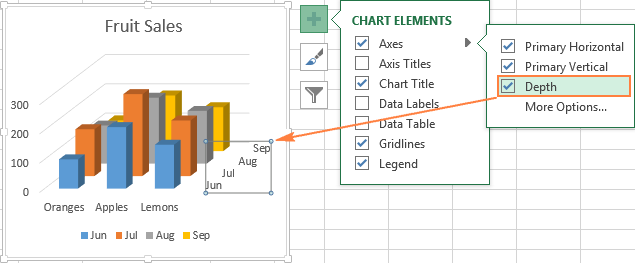
Plot Multiple Data Sets on the Same Chart in Excel ... Jun 29, 2021 · You can further format the above chart by making it more interactive by changing the “Chart Styles”, adding suitable “Axis Titles”, “Chart Title”, “Data Labels”, changing the “Chart Type” etc. It can be done using the “+” button in the top right corner of the Excel chart.

How to Make a Pie Chart in Excel & Add Rich Data Labels to The Chart!

Present your data in a doughnut chart - support.microsoft.com Click on the chart where you want to place the text box, type the text that you want, and then press ENTER. Select the text box, and then on the Format tab, in the Shape Styles group, click the Dialog Box Launcher . Click Text Box, and then under Autofit, select the Resize shape to fit text check box, and click OK.

How to make a pie chart in Excel

How to Make Pie of Pie Chart in Excel (with Easy Steps) Step-04: Employing Data Labels Format You can also make changes to data labels. Which will make your information more visual. At first, you have to click on the + icon. Then, from the Data Labels arrow >> you need to select More Options. At this time, you will see the following situation.

Lesson 2 | How to Create Charts Using Microsoft Excel Tutorial

How To Make A Pie Chart In Excel. - Spreadsheeto How To Make A Pie Chart In Excel. In Just 2 Minutes! Written by co-founder Kasper Langmann, Microsoft Office Specialist. The pie chart is one of the most commonly used charts in Excel. Why? Because it’s so useful 🙂. Pie charts can show a lot of information in a small amount of space. They primarily show how different values add up to a whole.

How to make a pie chart in Excel

Pie Chart in Excel - Inserting, Formatting, Filters, Data Labels Click on the Instagram slice of the pie chart to select the instagram. Go to format tab. (optional step) In the Current Selection group, choose data series "hours". This will select all the slices of pie chart. Click on Format Selection Button. As a result, the Format Data Point pane opens.

How to Make a PIE Chart in Excel (Easy Step-by-Step Guide)

How to display leader lines in pie chart in Excel? - ExtendOffice To display leader lines in pie chart, you just need to check an option then drag the labels out. 1. Click at the chart, and right click to select Format Data Labels from context menu. 2. In the popping Format Data Labels dialog/pane, check Show Leader Lines in the Label Options section. See screenshot: 3. Close the dialog, now you can see some ...

How to Make a PIE Chart in Excel (Easy Step-by-Step Guide)

How to Combine or Group Pie Charts in Microsoft Excel Click on the first chart and then hold the Ctrl key as you click on each of the other charts to select them all. Click Format > Group > Group. All pie charts are now combined as one figure. They will move and resize as one image. Choose Different Charts to View your Data

How to Make a Pie Chart in Excel & Add Rich Data Labels to The Chart!

Creating Pie Chart and Adding/Formatting Data Labels (Excel) Creating Pie Chart and Adding/Formatting Data Labels (Excel)

How to Make Pie Charts and Graphs in Excel - BSUPERIOR

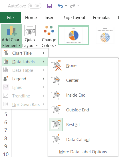
Excel Pie Chart - How to Create & Customize? (Top 5 Types) Step 1: Click on the Pie Chart > click the ' + ' icon > check/tick the " Data Labels " checkbox in the " Chart Element " box > select the " Data Labels " right arrow > select the " More Options… ", as shown below. The " Format Data Labels" pane opens.

Line Chart in Excel - Easy Excel Tutorial

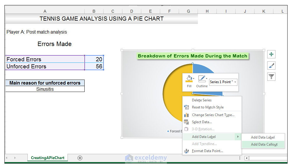
Add or remove data labels in a chart - support.microsoft.com Click the data series or chart. To label one data point, after clicking the series, click that data point. In the upper right corner, next to the chart, click Add Chart Element > Data Labels. To change the location, click the arrow, and choose an option. If you want to show your data label inside a text bubble shape, click Data Callout.

New, better alternative to Pie Charts: Treemap - Efficiency 365

How to Create and Format a Pie Chart in Excel - Lifewire Select the plot area of the pie chart. Right-click the chart. Select Add Data Labels . Select Add Data Labels. In this example, the sales for each cookie is added to the slices of the pie chart. Change Colors When a chart is created in Excel, or whenever an existing chart is selected, two additional tabs are added to the ribbon.

Excel charts: add title, customize chart axis, legend and data labels

Change the format of data labels in a chart To get there, after adding your data labels, select the data label to format, and then click Chart Elements > Data Labels > More Options. To go to the appropriate area, click one of the four icons ( Fill & Line, Effects, Size & Properties ( Layout & Properties in Outlook or Word), or Label Options) shown here.

Python matplotlib Pie Chart

How to add or move data labels in Excel chart? - ExtendOffice In Excel 2013 or 2016. 1. Click the chart to show the Chart Elements button . 2. Then click the Chart Elements, and check Data Labels, then you can click the arrow to choose an option about the data labels in the sub menu. See screenshot: In Excel 2010 or 2007. 1. click on the chart to show the Layout tab in the Chart Tools group. See ...

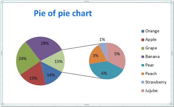
How to create pie of pie or bar of pie chart in Excel?

Comparison Chart in Excel | Adding Multiple Series Under Same ... This window helps you modify the chart as it allows you to add the series (Y-Values) as well as Category labels (X-Axis) to configure the chart as per your need. Under Legend Entries ( S eries) inside the Select Data Source window, you need to select the sales values for the year 2018 and year 2019.

How to Create a Pie Chart in Microsoft Excel

Create a multi-level category chart in Excel - ExtendOffice Create a multi-level category chart in Excel A multi-level category chart can display both the main category and subcategory labels at the same time. When you have values for items that belong to different categories and want to distinguish the values between categories visually, this chart can do you a favor.

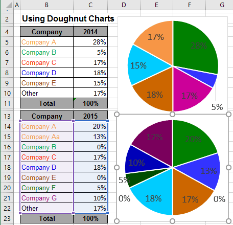
Using Pie Charts and Doughnut Charts in Excel

Create a Pie Chart in Excel (In Easy Steps) - Excel Easy Create the pie chart (repeat steps 2-3). 7. Click the legend at the bottom and press Delete. 8. Select the pie chart. 9. Click the + button on the right side of the chart and click the check box next to Data Labels. 10. Click the paintbrush icon on the right side of the chart and change the color scheme of the pie chart.

4.1 Choosing a Chart Type – Beginning Excel

How to Make a Pie Chart with Multiple Data in Excel (2 Ways) - ExcelDemy First, to add Data Labels, click on the Plus sign as marked in the following picture. After that, check the box of Data Labels. At this stage, you will be able to see that all of your data has labels now. Next, right-click on any of the labels and select Format Data Labels. After that, a new dialogue box named Format Data Labels will pop up.

Excel 3-D Pie charts - Microsoft Excel 2010

Everything You Need to Know About Pie Chart in Excel - SpreadsheetWeb How to Make a Pie Chart in Excel. Start with selecting your data in Excel. If you include data labels in your selection, Excel will automatically assign them to each column and generate the chart. Go to the INSERT tab in the Ribbon and click on the Pie Chart icon to see the pie chart types. Click on the desired chart to insert.

Share :